Process Capability: Definition and standard evaluation

Process Capability tells you, to what extent the process is likely to satisfy the customer's wish.
Process Capability evaluation compares:

• Customer's Specifications: Location and Variation
• Process Performance: Location and Variation

Standard Process Capability calculations assume 99.73% coverage of the process mapped as:
Where is the process mean and σ is the process standard deviation.

The standard evaluation of Process Capability Indices Cp & Cpk is given by the following formulae:
 

Where: USL = Upper Specification Limit LSL = Lower Specification Limit = Process Mean σ = Process standard deviation

A detailed treatment on computing the standard Process Capability indices is given by Dr. M M Kapadia¹ in his article on this web site: Measuring Your Process Capability.

What is described above is the standard practice of calculating Process Capability, and is practised widely. However there are often special situations that need to be addressed in a different way.

Unilateral tolerances:

One-sided tolerances impose only an upper limit or a lower limit on the process, and leave the specification unbounded on the other side.

Let us take an example of a motor shaft journal where the surface roughness needs to be maintained in the grinding operation. The design specification on the surface roughness is stated as '1.2µm Ra Maximum'. This means that the surface roughness should not exceed the value of 1.2µm in any of the shafts.

The Process Capability for this situation is often modelled as follows:

• USL = 1.2 (Stated Tolerance)
  
• LSL = 0

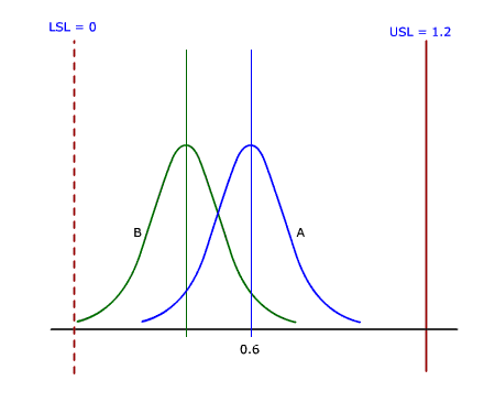
Such a definition of specifications leads to an erroneous evaluation of Process Capability. The figure shown here is based on specification limits of USL=1.2 and LSL=0. It compares the Process Capability of two processes for the characteristic of surface roughness. It can be seen from the figure that for the characteristic of surface roughness, Process B is better than Process A. However if you calculate the traditional way, the Process Capability of Process A shows up to be better. This has happened because a limit of 0 is imposed on the LSL. As the process leaves the artificially created center-of-specifications of 0.6, and gets closer to the lower limit, the process is actually penalized for getting better. Imposing a limit on the process where one does not exist is not a sound practice!

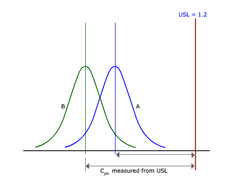
To overcome this fallacy, the Capability needs to be modelled as follows: USL = 1.2 LSL is not defined Cpk = CpkUpper = Cpu Cp is not defined Now the comparison of the two processes appears as shown in the adjacent figure. This evaluation reflects the correct picture of the Process Capability.

AIAG's SPC manual (2^nd edition, July 2005)² suggests an alternate evaluation of the Cp index for unilateral tolerances based on the physical limits imposed on the process. This implies that a surrogate lower limit of 0 is imposed in the above example process for the purpose of Capability evaluation. However, as pointed in the manual, the index C_p no more conveys the same meaning as it does in case of bilateral tolerances and does not maintain the same relationship with the C_pk index.

Computing an index C_p that conveys no useful information may be a waste of effort.

Non-Normal Distributions:

The standard process capability evaluation is based upon the assumption that the process under consideration is Normally distributed, as the assumption that covers 99.73% of the area under the process curve only applies for Normal distributions.

Applying the standard Process Capability evaluation formulae for processes irrespective of Normal distribution may lead to erroneous results.

There are two commonly used approaches used to evaluate the capability of Non-Normal processes.

• Data Transformation
• Evaluation of areas under Non-normal tails by fitting Other-than-Normal distributions.

Data Transformation:

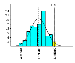
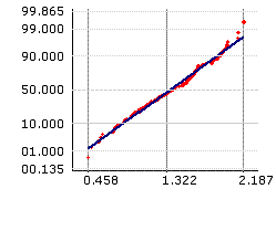
Transforms are applied on the available Non-Normal data to transform it to an equivalent Normal (or close-to-Normal) distribution that can be conveniently analyzed. There are two popularly used transformation methods to transform data to Normality.

• Box-Cox Transformation
• Johnson Transformation

Box-Cox Transformation

The Box-Cox transformation was proposed by George E. P. Box and David R. Cox³ in 1964.

The Box-Cox power transformation is expressed as

Y = y^λ when λ ≠ 0

Y = Log_ey when λ = 0

-5 ≤ λ ≤ +5

To determine the value of λ, for a good transformation, Box, Hunter and Hunter⁴ suggest that a standard analysis be done for various values of λ as follows:

is the Geometric Mean of the original data. The above model is recursively tested for several values of λ between -5 and +5. The maximum likelihood value of λ is the one for which the Residual Sum-of-Squares is minimum.

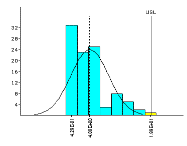
Once transformed, Normality of the transformed data is verified, and Process Capability Evaluation done on the transformed data. Box-Cox transformation can be done only on non-zero, positive data.

Box-Cox transformation is best done using computers. Most statistical software packages will offer Box-Cox transformation as a standard feature.

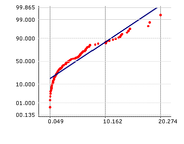Non-Normal Data for Assembly Gap
Box-Cox Transformation

Johnson Transformation

In 1949, Norman L. Johnson provided a system of transformations to transform Non-Normal data to a Normal form.

The Johnson system comprises of a family of three curves:

1. SB: Bounded
   
2. SL: Log Normal
   
3. SU: Unbounded

Nicholas R. Farnum (1996-97)⁵ has given a detailed description on the use of Johnson Curves. The Johnson system for the three curves that transforms data into a z distribution is expressed as

for the SU curves

for the SB curves

for the SL curves

Where:
Y is the transformed value
x is the variable to be transformed
is the Shape1 parameter
η is the Shape2 parameter
ε is the location parameter
λ is the scale parameter

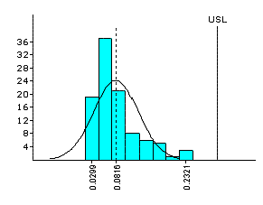
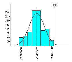
Decision rules have been formulated on selection of the SU, SB and SL curves for transformation of data. With fast computing power available at hand, an approach that is preferred is to transform the data recursively through several values of parameters and curve types. The transformation that gives a result that is closest to Normal is selected.

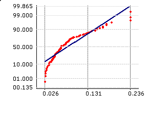Non-Normal Data on Run-out
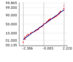Johnson Transformation modelled by a SU curve

Like the Box-Cox transformation, Johnson transformation is also best done using a suitable software.

A word of caution

Experts in the field have cautioned against using data transformations as above without adequately understanding implications of transformation. Donald Wheeler⁶ (1992) recommends that if the data is transformed for the purpose of convenient analysis, but results of an analysis need to be interpreted in terms of the original variable, the transformed data needs to be back-transformed. Giving results to an analyst in terms of transformed data conveys no useful information, since the transformed data is expressed in a scale and form (shape) that may be very different from the original data.

Actions for process improvement need to be taken on the basis of understanding of the process behavior. Process behavior can be best understood only if the data is back-transformed and expressed in familiar units. Back-transformation may apply to point estimates such as possible boundary values within which the process variation needs to be contained for achieving the target Process Capability. Process Capability indices however indicate probability of the process producing acceptable output, and do not require any back-transformation.

Data analysis by fitting Pearson curves

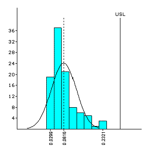
Analysis of non-normal data can be done by modeling of the data by an appropriate member from the Pearson distribution curves. Pearson curves were formulated by Karl Pearson in 1893. The observed data is analyzed and the measure of its Skewness (tendency of the peak to skew to the right or left) and Kurtosis (peaky or flat nature) is determined. A suitable Pearson curve with matching Skewness and Kurtosis is selected for modeling the data. An estimate of the area under the Pearson curve beyond the specification limits will help evaluate the Process Capability of the process under study. John A. Clements7(1989) has documented standardized tails (0.135 percentile and 99.865 percentile) and standardized medians (50 percentile) for Pearson family of curves. The method of evaluation of Process Capability on the basis of fitted Pearson curves is widely known as the Clements Method.

Parameter Value Mean (X-Bar) 0.081610 Std. Deviation (s) 0.047053 Skewness (Sk) 1.495375 Kurtosis (Ku) 2.108079 Percentiles: x50 (Median) 0.065258 x99865 0.283640 x00135 0.037001 Capability Statistic: Cp NA Cpl NA Cpu 1.0749 Cpk 1.0749

Concluding Remarks

Process Capability evaluation has gained wide acceptance around the world as a tool for Quality measurement and improvement. Standard formulae and quick calculation spreadsheets provide easy means of evaluating process capability. Process Capability evaluation should however not be done blindly, by plugging in available data into standard formulae. Special situations described above require appropriate methods of data evaluation to lead to correct conclusions about process behavior.

References:

1. M. M. Kapadia, "Measuring Your Process Capability", Symphony Technologies.
2. AIAG, "Statistical Process Control", Reference manual 2nd Edition, July 2005
3. Box, G. E. P. and Cox, D. R., "An analysis of transformations". Journal of Royal Statistical Society, Series B, vol. 26, 1964.
4. Box G. E. P., Hunter William G., Hunter J. Stuart, "Statistics for Experimenters, An introduction to Design, Data Analysis and Model building", 1978.
5. Nicholas R. Farnum, "Using Johnson Curves to Describe Non-Normal Data", Quality Engineering, 9 (2), 329- 336, (1996-97).
6. Donald J. Wheeler, "Understanding Statistical Process Control", Second Edition, 1992.
7. John A. Clements, "Process Capability Calculations for Non-Normal Distributions", Quality Progress, 95-100, September 1989.
8. Douglas C. Montgomery, "Introduction to Statistical Quality Control", 4th Edition, 2004.
9. Kotz Samuel & Lovelace Cynthia R., "Process Capability Indices in Theory and Practice", 1998.